Machine Learning Engineering - 01 - Intro
1. Introduction to Machine Learning
- Features: everything we know about the object.
- Target: what we want to predict
We collect all the features of all the objects we similar into a table, together with a column of the target.
Training means aking the features and the target and giving them to a machine learning algorithm. The algorithm produces a model.
The model encapsulates all the patterns it learned from the data. It is a single artifact we can save and use later.
Once we have the model, we can use it to predict the target for objects for which we don’t know the target. We take the features (all the information about an object except the target, because this is what we want to predict) put them into the model, and the model outputs the prediction.
The model is not always able to predict the exact target of a specific object. But the predictions are usually correct on average.
Let’s drill it into our heads: machine learning is a process of extracting patterns from data. The data consists of features (information about the object) and the target (what we want to predict). The output of machine learning is a model. To use it, we take the features of a new object, put them into the model, and get predictions of the target.
2. ML vs Rules-Based Systems
In a rules-based system, we create the rules ourselves and write them in code. The data and the code together form the software, and the software produces the outcome. The rules are hard-coded. Rules become hard to maintain in a complex problem. They are not suitable for complex problems.
Machine Learning is suitable for complex problems.
I have a post about the difference between “complicated” and “complex”. Look it up in this blog.
In machine learning, the roles flip. The outcome becomes an input to the machine learning algorithm (as targets in the training dataset), together with the features. The algorithm produces a model. Then, for cases where we don’t know the outcome (target), we take the data and the model, and the model produces the prediction (target).
One interesting realization: when migrating from a rules-based system to a ML system, the condition variables in a rules based system become features for a machine learning model.
So it might be a good idea to start with a rules-based system and not jump into ML immediately. This forces you to think about the rules which will becomes features for the ML system.
But this might be a double edged sword: you start the ML system with an unspoken or hidden or unconscious bias… Think about it. You are implicitly assuming that those specific properties (the variables of the conditions in the rules-based system) are the ones that matter (by making them features in the training dataset), and you have excluded the other properties of the objects. This is Historical Bias and Omitted Variable Bias.
3. Supervised ML
Supervised machine learning is a subfield of artificial intelligence where a model is trained on a labeled dataset, meaning each training input is paired with its correct, corresponding output.
The algorithm analyzes this training data to learn an underlying mapping function ($f(x) = y$). Once fully trained, the model applies this learned function to accurately predict outcomes or classify new, unseen data.
The data we train the model on has two parts:
- The features matrix, usually written as capital X: $X$. In a simple 2 dimensional matrix, we have an array where the rows are our observations (the objects we want to make predictions for), and the columns are the features.
- The target variable, usually written as lowercase y: $y$. It is a vector: a 1 dimensional array of numbers.
We input the feature matrix $X$ and target vector $y$ into a machine learning algorithm to train the model. The model is usually denoted as lowercase function g: $g$. This function takes $X$ as input and outputs a prediction, $\hat{y}$, that is approximately equal to the true target $y$.
\[g(X) = \hat{y} \approx y\] \[g(X) \approx y\]The goal of supervised learning is to come up with a $g()$ such that when we apply it to $X$, the output $\hat{y}$ is as close as possible to the target variable $y$. The process of finding $g$ is called training.
Types of Supervised ML
Based on what $g$ outputs and what the target variable looks like, there are different types of supervised machine learning.
Regression
Predicting a continuous numerical value (e.g., estimating a house price based on its square footage).
Classification
Predicting a discrete categorical label (e.g., determining if an email is Spam or Not Spam).
- Binary classification: 2 categories, e.g. spam detection (hotdog, not hotdog)
- Multiclass classification: more than 2 categories, e.g. classifying images into cats, dogs and cars.
Ranking
Also called Learning to Rank or LTR.
Predicting the optimal order of a list of items based on their relevance to a specific context or query.
Unlike classification (which predicts a label) or regression (which predicts a continuous score for a single item in isolation), ranking algorithms optimize the relative positions of an entire group of items. The model is trained on data where the inputs are queries and lists of items, and the labels are the correct orderings or explicit relevance scores (e.g., 0 for irrelevant, 2 for highly relevant).
This is used in search engines and recommendation systems.
4. CRISP-DM
CRISP-DM stands for Cross-Industry Standard Process for Data Mining, a widely used cyclical framework that guides data science and analytics projects from start to finish.
It is basically Agile but for the unpredictable nature of data science. You can use both at the same time: Agile to manage the daily tasks, meetings, and timelines, and using CRISP-DM as the map to guide the technical data exploration and modeling steps.
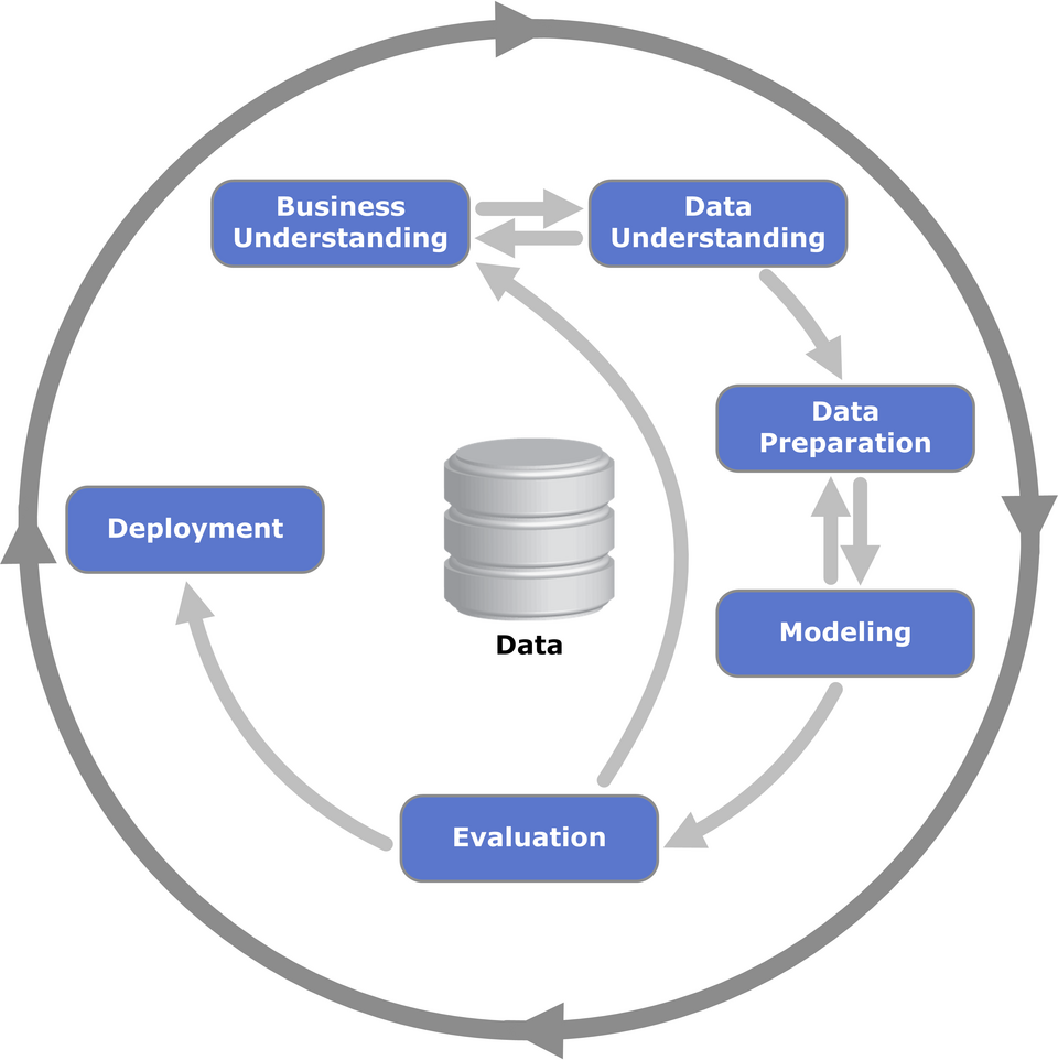
- Business Understanding: Learn what the business needs, define goals, and plan the project.
- Data Understanding: Gather initial data, check its quality, and find early insights.
- Data Preparation: Clean the data, fix errors, and format it for the models. This phase often takes the most time.
- Modeling: Choose and apply machine learning or statistical techniques to the data.
- Evaluation: Test how well the model works and check if it meets business goals.
- Deployment: Put the final model into action, monitor its performance, and plan future updates.
5. Model Selection Process
Simulating future data with a Validation Set
To evaluate the model, we take the dataset, put aside a small part of it (say 20%) and pretend this part doesn’t exist. We train on the remaining 80% only. The held-out part is what we evaluate against. We call it the validation set.
From the training set we extract the feature matrix $X$ and the target $y$, and we train the model $g$ using only these. From the validation set we extract another matrix, $X_v$, and its target $y_v$: the model has never seen them during training.
We apply $g$ to $X_v$ and get predictions. Because the output is a probability, we first convert the predictions into the final decisions. For example, if the probability is greater than 0.5 we predict hotdog, otherwise not hotdog (in binary classification). Then we compare the predicted values with the actual values of $y_v$ (actually hotdog or not hotdig) and count in how many cases the model was correct. If it was correct in 4 out of 6 cases, its accuracy is 66%.
The Multiple Comparisons Problem (MCP)
Which model to choose? logistic regression? Decision tree? neural network? …?
The multiple comparisons problem (also known as the multiplicity problem) occurs when we evaluates multiple models on the same dataset, heavily inflating the risk of false-positive discoveries.
How it manifests:
- Hyperparameter Tuning and Model Selection: If you evaluate variations on the same validation or test set, the configuration that achieves the highest accuracy might not actually be the best model. It may simply be the model that got lucky and “overfitted” to the random noise inherent in that specific data split.
- Test Set Reuse (Data Leakage): If you repeatedly tweak a model, evaluate it on the test set, and use that feedback to tweak it again, the test set is no longer an independent evaluator. Across many iterations (comparisons), the model’s performance metrics become optimistically biased and unrepresentative of true real-world data.
- Feature selection (data dredging): Imagine you test 100 useless features to see if they predict your target. If you use a standard 5% error rule, 5 of those features will look useful purely by random luck. If you do not fix this mathematically, you will pick features that are just meaningless random noise, leading to a broken model that fails on new data.
- A/B/n Testing and Multi-Arm Bandits: Tracking 10 different metrics across 5 demographic segments yields 50 separate statistical comparisons. The probability of seeing a “statistically significant” improvement purely by chance skyrockets.
So how do we mitigate this problem?
We split the dataset into 3 distinct sets:
- Training set
- Validation set
- Test set
By separating your data, you create strict firewalls that stop you from cheating:
- The Validation Set protects the Training Set. You can test 1,000 different hyperparameter combinations on the validation set. Even if the “winning” model just got lucky, the training data remains untainted.
- The Test Set protects the Validation Set. Once you pick your final model, you test it one single time on the test set. Because this data was never used to make any decisions or comparisons, its final score is a true, unbiased reflection of real-world performance.
What this does not protect against is the feature selection problem: if you have 10,000 features and you search for correlations using only your training set, you will still accidentally select hundreds of useless, noisy features purely by random chance. Because those “lucky” features are present in the training, validation, and test sets, your model will be forced to use fake rules built on noise. When you finally test those rules on unseen data, the “luck” runs out, and your model’s accuracy will completely crash. The mitigation here is to use statistical adjustments like the Bonferroni correction or False Discovery Rate (FDR) to filter out features that just got lucky.
Note that it is possible to reuse the validation data. After selecting the best model, the validation and training datasets can be combined to form a single training dataset for the chosen model before testing it on the test set. This is standard practice.
6. Introduction to NumPy
https://www.datacamp.com/cheat-sheet/numpy-cheat-sheet-data-analysis-in-python
7. Linear Algebra Refresher
Vector Operations
\[2 \cdot \begin{bmatrix} 2 \\ 4 \\ 5 \\ 6 \end{bmatrix} = \begin{bmatrix} 2 \cdot 2 \\ 2 \cdot 4 \\ 2 \cdot 5 \\ 2 \cdot 6 \end{bmatrix} = \begin{bmatrix} 4 \\ 8 \\ 10 \\ 12 \end{bmatrix}\]>>> u = np.array([2, 4, 5, 6])
>>> 2 * u
array([ 4, 8, 10, 12])
>>> v = np.array([1, 0, 0, 2])
>>> u + v
array([3, 4, 5, 8])
Vector-Vector Multiplication (dot product)
\[\mathbf{u} \cdot \mathbf{v} = \sum_{i=1}^{n} u_i v_i = \begin{bmatrix} 2 \\ 4 \\ 5 \\ 6 \end{bmatrix} \cdot \begin{bmatrix} 1 \\ 0 \\ 0 \\ 2 \end{bmatrix} = (2 \cdot 1) + (4 \cdot 0) + (5 \cdot 0) + (6 \cdot 2) = 14\]However we usually write the first vector as a horizontal row vector to show it multiplying into the vertical column vector:
\[\mathbf{u}^T \mathbf{v} = \sum_{i=1}^{n} u_i v_i = \begin{bmatrix} 2 & 4 & 5 & 6 \end{bmatrix} \begin{bmatrix} 1 \\ 0 \\ 0 \\ 2 \end{bmatrix} = 2(1) + 4(0) + 5(0) + 6(2) = 14\]def vector_vector_multiplication(u, v):
assert u.shape[0] == v.shape[0]
n = u.shape[0]
result = 0.0
for i in range(n):
result = result + u[i] * v[i]
return result
>>> vector_vector_multiplication(u, v)
14.0
With NumPy, we have to use the dot function, and not u * v which would give array([ 2, 0, 0, 12])
>>> u.dot(v)
14
Matrix-Vector Multiplication
\[\mathbf{U}\mathbf{v} = \begin{bmatrix} 2 & 4 & 5 & 6 \\ 1 & 2 & 1 & 2 \\ 3 & 1 & 2 & 1 \end{bmatrix} \begin{bmatrix} 1 \\ 0 \\ 0 \\ 2 \end{bmatrix} = \begin{bmatrix} \mathbf{u}_0^T \mathbf{v} \\ \mathbf{u}_1^T \mathbf{v} \\ \mathbf{u}_2^T \mathbf{v} \end{bmatrix} = \begin{bmatrix} (2 \cdot 1) + (4 \cdot 0) + (5 \cdot 0) + (6 \cdot 2) \\ (1 \cdot 1) + (2 \cdot 0) + (1 \cdot 0) + (2 \cdot 2) \\ (3 \cdot 1) + (1 \cdot 0) + (2 \cdot 0) + (1 \cdot 2) \end{bmatrix} = \begin{bmatrix} 14 \\ 5 \\ 5 \end{bmatrix}\]>>> U = np.array([
... [2, 4, 5, 6],
... [1, 2, 1, 2],
... [3, 1, 2, 1],
... ])
>>> U.shape
(3, 4)
def matrix_vector_multiplication(U, v):
    assert U.shape[1] == v.shape[0]

    num_rows = U.shape[0]

    result = np.zeros(num_rows)

    for i in range(num_rows):
        result[i] = vector_vector_multiplication(U[i], v)

    return result
>>> matrix_vector_multiplication(U, v)
array([14.,  5.,  5.])
>>> U.dot(v)
array([14,  5,  5])
Matrix-Matrix Multiplication
\[\mathbf{U}\mathbf{V} = \begin{bmatrix} 2 & 4 & 5 & 6 \\ 1 & 2 & 1 & 2 \\ 3 & 1 & 2 & 1 \end{bmatrix} \begin{bmatrix} 1 & 1 & 2 \\ 0 & 0.5 & 1 \\ 0 & 2 & 1 \\ 2 & 1 & 0 \end{bmatrix} = \begin{bmatrix} \vert & \vert & \vert \\ \mathbf{U}\mathbf{v}_0 & \mathbf{U}\mathbf{v}_1 & \mathbf{U}\mathbf{v}_2 \\ \vert & \vert & \vert \end{bmatrix} = \begin{bmatrix} 14 & 20 & 13 \\ 5 & 6 & 5 \\ 5 & 8.5 & 9 \end{bmatrix}\]>>> V = np.array([
... [1, 1, 2],
... [0, 0.5, 1],
... [0, 2, 1],
... [2, 1, 0],
... ])
def matrix_matrix_multiplication(U, V):
    assert U.shape[1] == V.shape[0]

    num_rows = U.shape[0]
    num_cols = V.shape[1]

    result = np.zeros((num_rows, num_cols))

    for i in range(num_cols):
        vi = V[:, i]
        Uvi = matrix_vector_multiplication(U, vi)
        result[:, i] = Uvi

    return result
>>> matrix_matrix_multiplication(U, V)
array([[14. , 20. , 13. ],
       [ 5. ,  6. ,  5. ],
       [ 5. ,  8.5,  9. ]])
In NumPy we just use the dot function:
>>> U.dot(V)
array([[14. , 20. , 13. ],
       [ 5. ,  6. ,  5. ],
       [ 5. ,  8.5,  9. ]])
Identity Matrix
The identity matrix is a square matrix where on the diagonal we have ones, and zeros everywhere else. It is denoted as capital I: $I$.
\[\mathbf{I}_n = \begin{bmatrix} 1 & 0 & \cdots & 0 \\ 0 & 1 & \cdots & 0 \\ \vdots & \vdots & \ddots & \vdots \\ 0 & 0 & \cdots & 1 \end{bmatrix}\] \[\mathbf{I} = \begin{bmatrix} 1 & 0 & 0 \\ 0 & 1 & 0 \\ 0 & 0 & 1 \end{bmatrix}\]To create an Identity matrix, we use the NumPy function eye:
>>> I = np.eye(3)
>>> I
array([[1., 0., 0.],
       [0., 1., 0.],
       [0., 0., 1.]])
For any matrix $A$:
\[\mathbf{I}\mathbf{A} = \mathbf{A}\mathbf{I} = \mathbf{A}\]It is like multiplying by the number 1.
>>> V.dot(I)
array([[1. , 1. , 2. ],
       [0. , 0.5, 1. ],
       [0. , 2. , 1. ],
       [2. , 1. , 0. ]])
Notice that $V$ is rectangular: 3 columns by 4 rows.
The sizes of the identity matrices must change depending on which side they are placed:
\[\mathbf{I}_m \mathbf{U}_{m \times n} = \mathbf{U}_{m \times n} \mathbf{I}_n = \mathbf{U}_{m \times n}\]$m$ being the number of rows, and $n$ being the number of columns.
Inverse
For any square, invertible matrix $A$, multiplying it by its inverse ${A}^{-1}$ always results in the identity matrix $I$. Just like the identity property, the order of multiplication does not matter.
Only perfectly square matrices $m = n$ can have a true inverse.
\[\mathbf{A} \mathbf{A}^{-1} = \mathbf{A}^{-1} \mathbf{A} = \mathbf{I}\]>>> Vs = V[[0, 1, 2]]
>>> Vs
array([[1. , 1. , 2. ],
[0. , 0.5, 1. ],
[0. , 2. , 1. ]])
To compute the inverse we use a method from NumPy called inv. It lives in the linalg package (linear algebra):
>>> Vs_inv = np.linalg.inv(Vs)
>>> Vs_inv
array([[ 1.        , -2.        ,  0.        ],
       [ 0.        , -0.66666667,  0.66666667],
       [ 0.        ,  1.33333333, -0.33333333]])
>>> Vs_inv.dot(Vs)
array([[1., 0., 0.],
       [0., 1., 0.],
       [0., 0., 1.]])
8. Introduction to Pandas
https://www.datacamp.com/cheat-sheet/pandas-cheat-sheet-for-data-science-in-python
9. Let’s Practice
You can find the dataset and the jupyter notebook here.
Dataset: here.
Jupyter notebook: here, and you can view it below:
Privacy-First Subscription
Receive a notification in your inbox whenever I publish a new post. This is a reader-focused subscription loop built for absolute privacy: you stay in control, and I do not see, track, or collect your email address.
Follow via FeedRabbit