Demystifying JupyterLab
More than 10 years ago, right around the migration of Python from v2 to v3, I played a lot with Numpy, Pandas and Matplotlib. So I had to toy around with Jupyter. But since then I didn’t need to use it.
This post is to refresh my Jupyer skills and get up to date.
I won’t cover all of it. I am interested only in how it fits in my way of working.
A Little Bit of History
I like to understand the history of things because it explains why some things are the way they are. Without this context, a lot of architecture or design decisions seem odd.
The notebook interface that exists today is the result of 3 distinct generations:
IPython Notebook (2011) -> Jupyter Notebook (2014) -> JupyterLab (2018)
Gen1: IPython Notebook
Launched in 2011, the original IPython Notebook revolutionized programming by moving execution from a rigid terminal into a dynamic web browser window. The acronym stood for “Interactive Python”. For the first time, developers could run fragments of Python code sequentially, save the outputs visually, and write accompanying text. Because of this history, all Jupyter notebook files still use the .ipynb file extension.
So that resolves the mystery of why the file extension is that way.
Gen2: Jupyter Notebook (Multilingual Rebrand)
By 2014, the open-source community realized that this modular, cell-based format was incredibly powerful for languages beyond just Python. The project spun out into Project Jupyter, a portmanteau representing the three core languages it initially targeted: Julia, Python, and R. The classic Jupyter Notebook dashboard allowed users to view local directories and spin up standalone notebook tabs in their browser.
Gen3: JupyterLab
While the classic notebook interface was groundbreaking, working across multiple files was cumbersome because every single notebook opened in a brand-new browser tab. To fix this, JupyterLab was introduced in 2018. It acts like a full-featured web-based IDE. Inside a single browser tab, JupyterLab provides a complete tabbed interface, interactive file sidebars, built-in terminal consoles, and side-by-side notebook views.
The Many Ways to Set Up and Run Jupyter
A. Cloud-Based Without Installation
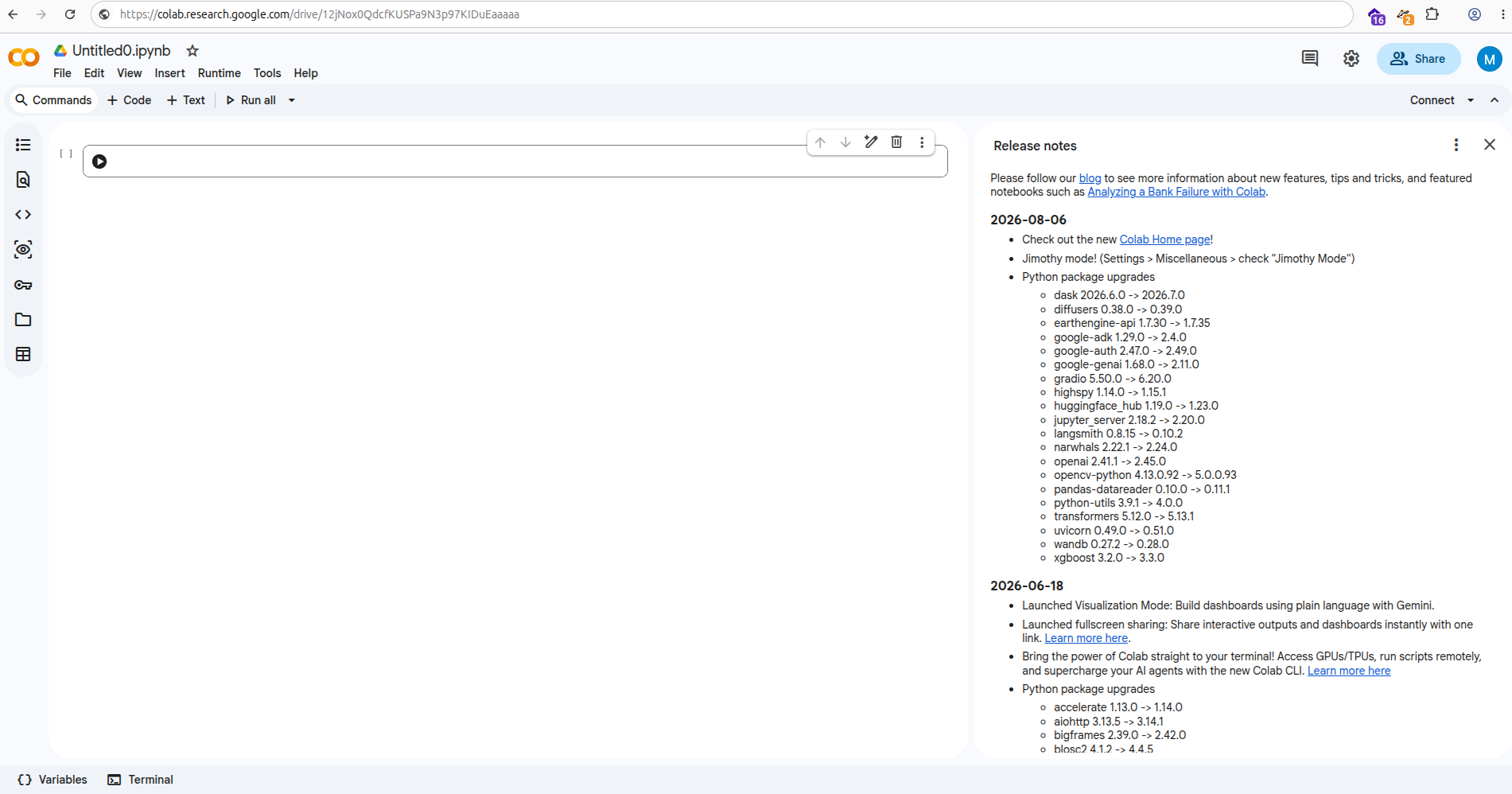
- Google Colab: Just go to https://colab.research.google.com/ and you’ll see the “New notebook” button. You click it and your environment is ready. Can’t get easier than this.
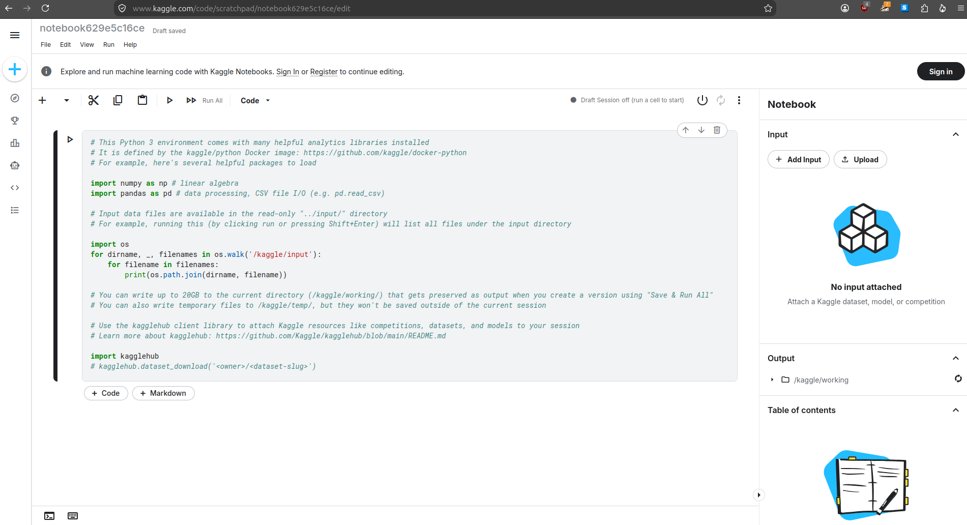
- Kaggle Notebooks: This is optimized for completing Kaggle challenges. Just go to https://www.kaggle.com/code and click on “New Notebook”. Easy.
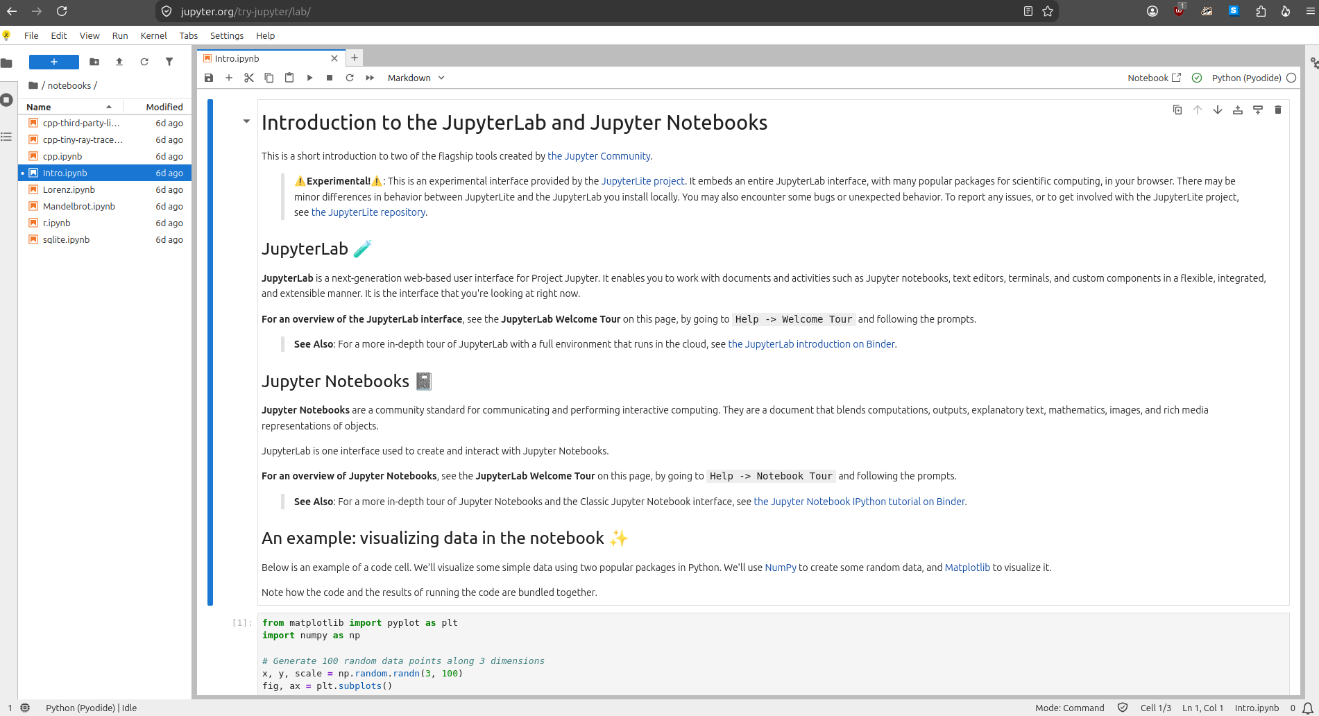
- Jupyter Try: Go to https://jupyter.org/try and click on “JupyerLab” and you’re good to go.
B. Local Graphical Installers
- Anaconda Desktop (replaces Anaconda Navigator): https://www.anaconda.com/docs/anaconda-desktop/key-features. Not for me, but might be for you.
C. CLI
This is the modular way.
I do not use pip anymore (willingly), but leaving the commands here so that they are clear for everybody.
- Classic Notebook (old):
- Install:
pip install notebook - Launch:
jupyter notebook
- Install:
- JupyterLab:
- Install:
pip install jupyterlab - Launch:
jupyter lab
- Install:
D. Code Editor Integration
Instead of running an interface inside an internet browser window, you can plug you computational notebook engines straight into the IDE via the Jupyter extension: https://marketplace.visualstudio.com/items?itemName=ms-toolsai.jupyter.
The Architecture: UI vs Engine
To use the local setup, it is crucial to understand the structural difference between the UI and the Execution Engine.
When you write a line of code inside a notebook cell and press Shift + Enter, the interface you are looking at cannot actually compute the mathematical equations. It requires a backend interpreter to do the work:
ipykernelis the engine. It is an invisible background utility that processes raw Python strings, carries out instructions on your processor, tracks variable states, and passes the output text or graph data back up.- VS Code, JupyterLab, and Jupyter Notebook are the screens. They handle text formatting, keyboard shortcuts, extension layouts, and code coloring.
So the flow looks something like this:
UI (VSCode Jupyter Extension, JupyterLab, or Classic Notebook) –> sends code cells –> Execution Engine (ipykernel) –> Executes code natively –> Local env (Python interpreter and packages).
How to set it up via the CLI
I personally use uv. So I am witing this to suit my workflow.
If I want to run a temporary ad-hoc notebook session to try something quickly, I just run this: uvx jupyter lab.
uvx fetches JupyterLab into an isolated ephemeral cache, spins up the browser dashboard instantly, and wipes the cached footprint clean when you close the session.
If I want to build a persistent workspace folder with its own isolated virtual environment, I go through the usual flow that I documented in a previous post: Rustification of Python - uv, ruff, ty - Automating Book Availability Checks.
These commands assume using the Jupyter extension for VSCode, and hence we install only the Jupyter engine:
# Initialize a structured project directory
uv init my-data-project && cd my-data-project

# Spin up an isolated virtual environment
uv venv

# Add only the vital background engine dependency
uv add --dev ipykernel
But what about conda?
I do not use it (willingly). Too slow and more commands to memorize. uv is fast and does everything I need. I see no reason to go back to conda or miniconda.
What if I install jupyterlab instead of ipykernel while using the Jupter extension for VSCode?
It will still work because ipykernel is a foundational structural dependency of JupyterLab. It’s just that you’re putting in there more stuff than needed.
Cheat Sheet
Let’s apply Pareto’s principle to unlock 80% of the tool’s power with 20% of the effort.
The Modes
- COMMAND MODE (Press
Esc)- Border indicator is BLUE
- Keyboard controls the layout
- examples: Add, Delete, Move cells
- EDIT MODE (Press
Enter)- Border indicator is GREEN
- Keyboard writes raw code/text
- Active cursor inside cell
Keyboard shortcuts
This is a matter of muscle memory…
- Environment control (in Command Mode)
A: Insert a new cell Above the current cell.B: Insert a new cell Below the current cell.D+D(Press D twice): Delete the selected cell.M: Change the cell type to Markdown (for documentation).Y: Change the cell type back to Code (for execution).Z: Undo the last cell deletion. For your “oops, I did it again” moments.Shift+Up/Down Arrow: Select multiple cells at once to move or delete them together.
- Execution Control (In either mode)
Shift+Enter: Run the active cell and automatically jump focus to the next cell below.Ctrl+Enter: Run the active cell and keep focus locked on that exact same cell.Alt+Enter(orOption+Enteron Mac): Run the active cell and immediately spawn a brand new cell right below it.
Magic Commands
I did not choose the name. Yes, they called them “magic commands”: https://ipython.readthedocs.io/en/stable/interactive/magics.html.
These let you control the notebook system or run terminal utilities directly inside a Python cell.
%matplotlib inline: Ensures all graphs, charts, and plots render instantly and cleanly directly beneath your code cells.%timeit [your statement]: Runs a specific line of code thousands of times in a micro-second loop to output the exact average processing speed. Great for optimizing slow code.%%time: Place this at the absolute top of a cell. When executed, it prints exactly how many seconds or milliseconds the entire cell took to run.%pwd: Prints the exact local folder directory path where your notebook is currently saved on your computer.! [terminal command]: Preceding any line with an exclamation mark allows you to execute raw system terminal commands without leaving the notebook. (e.g., !pip install pandas or !ls).
Interface Hacks
The real power of JupyterLab over the classic legacy notebook interface lies in its multi-window desktop fluidity.
- The Split-Screen drag: Click and hold the top tab of any open notebook file, then drag it to the left, right, or bottom of your browser window. JupyterLab will instantly split your workspace, allowing you to view an output chart on the right while writing data code on the left.
- New Console for Notebook: Right-click anywhere inside an open notebook and select “New Console for Notebook”. This opens an independent interactive scratchpad terminal on the side linked to the exact same execution engine. You can test experimental variables here without cluttering your primary report.
- Toggle the Sidebar (
Ctrl+B): Hide the file browser navigation tree to free up screen real estate for your code. Same key combo to unhide it. - The Universal Command Palette (
Ctrl+Shift+C): If you ever forget a keyboard shortcut or want to change JupyterLab to Dark Mode, open this palette and search for what you want to do using conversational English.
Presenting to Non-Technical Stakeholders
Jupyter comes with a native conversion engine called nbconvert that transforms your working scratchpad into polished, universally readable formats.
Navigate to File > Save and Export Notebook As…. You will see a dropdown list of conversion profiles: HTML, PDF, Markdown.
Another alternative is to hide the code cells: Select a cell containing code > In JupyterLab’s right-hand sidebar, click the Property Inspector icon (the small gears or settings cog) > Under Cell Metadata or Advanced Tools, you can add tag exclusions, or simply click the active button to collapse and hide the code input entirely, leaving only the chart output visible.
Some Useful JupyterLab Extensions
- Coding assistance: https://github.com/jupyter-lsp/jupyterlab-lsp
- Git version control directly in the left side panel: https://github.com/jupyterlab/jupyterlab-git
Privacy-First Subscription
Receive a notification in your inbox whenever I publish a new post. This is a reader-focused subscription loop built for absolute privacy: you stay in control, and I do not see, track, or collect your email address.
Follow via FeedRabbit